[ 딥러닝 코드 리뷰 - PRMI Lab ] - DDPM 코드 리뷰 및 실행

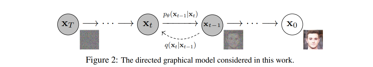
이번에는 DDPM 공식 레포 코드를 분석하고 그 안에 구현된 디테일들이나 최신 기술들에 대해 알아보려고합니다. 마지막에는 직접 돌려봐서 celeba 데이터셋에 대해서 훈련시키고 샘플링시키는 작업까지 해보겠습니다.

논문 링크: https://arxiv.org/pdf/2006.11239

 

U-Net

model

class Unet(Module):
    def __init__(
        self,
        dim,
        init_dim = None,
        out_dim = None,
        dim_mults = (1, 2, 4, 8),
        channels = 3,
        self_condition = False,
        learned_variance = False,
        learned_sinusoidal_cond = False,
        random_fourier_features = False,
        learned_sinusoidal_dim = 16,
        sinusoidal_pos_emb_theta = 10000,
        dropout = 0.,
        attn_dim_head = 32,
        attn_heads = 4,
        full_attn = None,    # defaults to full attention only for inner most layer
        flash_attn = False
    ):
        super().__init__()

        # determine dimensions

        self.channels = channels
        self.self_condition = self_condition
        input_channels = channels * (2 if self_condition else 1)

        # init_dim이 없으면 dim으로 
        init_dim = default(init_dim, dim)
        self.init_conv = nn.Conv2d(input_channels, init_dim, 7, padding = 3)

        # [dim, dim, dim * (dim_mults)[0], dim * (dim_mults)[1], ..., (dim_mults)[len(dim_mults) - 1]]
        # [64, 64, 128, 256, 512]
        dims = [init_dim, *map(lambda m: dim * m, dim_mults)]
        in_out = list(zip(dims[:-1], dims[1:]))

        # time embeddings

        time_dim = dim * 4

        self.random_or_learned_sinusoidal_cond = learned_sinusoidal_cond or random_fourier_features

        # time embedding(positional encoding)을 위한 SinusoidalPosEmb 생성.
        if self.random_or_learned_sinusoidal_cond:
            sinu_pos_emb = RandomOrLearnedSinusoidalPosEmb(learned_sinusoidal_dim, random_fourier_features)
            fourier_dim = learned_sinusoidal_dim + 1
        else:
            sinu_pos_emb = SinusoidalPosEmb(dim, theta = sinusoidal_pos_emb_theta)
            fourier_dim = dim

        # 선언한 sinu_pos_emb를 time_mlp에 추가 --> Linear --> GELU --> Linear
        self.time_mlp = nn.Sequential(
            sinu_pos_emb,
            nn.Linear(fourier_dim, time_dim),
            nn.GELU(),
            nn.Linear(time_dim, time_dim)
        )

        # attention

        if not full_attn:
            full_attn = (*((False,) * (len(dim_mults) - 1)), True)

        num_stages = len(dim_mults)
        full_attn  = cast_tuple(full_attn, num_stages)
        attn_heads = cast_tuple(attn_heads, num_stages)
        attn_dim_head = cast_tuple(attn_dim_head, num_stages)

        assert len(full_attn) == len(dim_mults)

        # prepare blocks

        FullAttention = partial(Attention, flash = flash_attn)
        resnet_block = partial(ResnetBlock, time_emb_dim = time_dim, dropout = dropout)

        # layers

        self.downs = ModuleList([])
        self.ups = ModuleList([])
        num_resolutions = len(in_out)


        # Down-sampling (downs)
        for ind, ((dim_in, dim_out), layer_full_attn, layer_attn_heads, layer_attn_dim_head) in enumerate(zip(in_out, full_attn, attn_heads, attn_dim_head)):
            is_last = ind >= (num_resolutions - 1)

            attn_klass = FullAttention if layer_full_attn else LinearAttention

            self.downs.append(ModuleList([
                resnet_block(dim_in, dim_in),
                resnet_block(dim_in, dim_in),
                attn_klass(dim_in, dim_head = layer_attn_dim_head, heads = layer_attn_heads),
                Downsample(dim_in, dim_out) if not is_last else nn.Conv2d(dim_in, dim_out, 3, padding = 1)
            ]))

        # Mid block
        mid_dim = dims[-1]
        self.mid_block1 = resnet_block(mid_dim, mid_dim)
        self.mid_attn = FullAttention(mid_dim, heads = attn_heads[-1], dim_head = attn_dim_head[-1])
        self.mid_block2 = resnet_block(mid_dim, mid_dim)

        # Up-sampling (ups)
        for ind, ((dim_in, dim_out), layer_full_attn, layer_attn_heads, layer_attn_dim_head) in enumerate(zip(*map(reversed, (in_out, full_attn, attn_heads, attn_dim_head)))):
            is_last = ind == (len(in_out) - 1)

            attn_klass = FullAttention if layer_full_attn else LinearAttention

            self.ups.append(ModuleList([
                resnet_block(dim_out + dim_in, dim_out),
                resnet_block(dim_out + dim_in, dim_out),
                attn_klass(dim_out, dim_head = layer_attn_dim_head, heads = layer_attn_heads),
                Upsample(dim_out, dim_in) if not is_last else  nn.Conv2d(dim_out, dim_in, 3, padding = 1)
            ]))

        default_out_dim = channels * (1 if not learned_variance else 2)
        self.out_dim = default(out_dim, default_out_dim)

        self.final_res_block = resnet_block(init_dim * 2, init_dim)
        self.final_conv = nn.Conv2d(init_dim, self.out_dim, 1)

    @property
    def downsample_factor(self):
        return 2 ** (len(self.downs) - 1)
    
    # DDPM의 reverse process과정
    def forward(self, x, time, x_self_cond = None):
        assert all([divisible_by(d, self.downsample_factor) for d in x.shape[-2:]]), f'your input dimensions {x.shape[-2:]} need to be divisible by {self.downsample_factor}, given the unet'

        if self.self_condition:
            x_self_cond = default(x_self_cond, lambda: torch.zeros_like(x))
            x = torch.cat((x_self_cond, x), dim = 1)

        x = self.init_conv(x)
        r = x.clone()

        t = self.time_mlp(time)

        h = []

        for block1, block2, attn, downsample in self.downs:
            x = block1(x, t)
            h.append(x)

            x = block2(x, t)
            x = attn(x) + x
            h.append(x)

            x = downsample(x)

        x = self.mid_block1(x, t)
        x = self.mid_attn(x) + x
        x = self.mid_block2(x, t)

        for block1, block2, attn, upsample in self.ups:
            x = torch.cat((x, h.pop()), dim = 1)
            x = block1(x, t)

            x = torch.cat((x, h.pop()), dim = 1)
            x = block2(x, t)
            x = attn(x) + x

            x = upsample(x)

        x = torch.cat((x, r), dim = 1)

        x = self.final_res_block(x, t)

        # 해당 값이 predicted noise값값
        return self.final_conv(x)

 

Unet에 대해서는 다 아실거라고 생각하고 간단히 정리하겠습니다.

•  x_self_cond
  • 이는 이전 출력을 다음 입력에 추가해서 넣어주기 위한 인자입니다.
• init_conv
  • input_channels -> init_dim으로 차원 embedding을 해주는 시작 convolution입니다.
• dims
  • dim_mults로 U-net의 downsample 차원을 조절해줍니다.
  • dim_mults가 (1, 2, 4, 8) 이면 [init_dim, init_dim*1, init_dim*2, init_dim*4, init_dim*8]
• time_dim
  • ddpm에서 현재 timestep T를 Unet의 input으로 넣어주는데, 이에 대한 embedding 크기를 나타냅니다.
• random_or_learned_sinusoidal_cond
  • positional embedding을 학습시킬것인지에 대한 인자입니다.
• time_mlp
  • Linear -> GELU -> Linear로 우리가 원하는 크기의 time embedding을 만듭니다.
• FullAttention
  • Unet에서 Attention을 사용하기 위해 정의한 부분입니다. (class Attention)
    • flash = flash_attn을 주어 더 빠른 flash attention을 수행시켜줄 수 있습니다. (저는 4090에서 flash attention을 지원하지 않아 못돌렸습니다.)
• downs, ups
  • ModuleList들을 저장한 배열인데, downs에는 resnet_block -> resnet_block -> attn_klass -> downsample을 저장해줍니다. 
  • forward()에서 downs배열을 for돌아서 넣고 mid_block 후에 ups배열 다 돈다음에 끝납니다.
  • 참고로 time embedding과 추가로 concatenate해서 돌리기 때문에, 배열의 차원이 기존과는 다릅니다.
    • class ResNetBlock을 참고하시면 될거 같습니다.

Attention, Positional Encoding과 관련된 부분은 설명하지 않겠습니다. Attention부분은 eipons 라이브러리로 대부분이 구현되어 있으며, mem key_value 를 사용하여 메모리 효율성을 높인 구현체입니다. 궁금하면 class Attention(full_attn)과 LinearAttention을 보시기 바랍니다. Positional Encoding은 이전의 NeRF code 분석글을 참고하시기 바랍니다.

 

GaussianDiffusion

class GaussianDiffusion(Module):
    def __init__(
        self,
        model,
        *,
        image_size,
        timesteps = 1000,
        sampling_timesteps = None,
        objective = 'pred_v',
        beta_schedule = 'sigmoid',
        schedule_fn_kwargs = dict(),
        ddim_sampling_eta = 0.,
        auto_normalize = True,
        offset_noise_strength = 0.,  # https://www.crosslabs.org/blog/diffusion-with-offset-noise
        min_snr_loss_weight = False, # https://arxiv.org/abs/2303.09556
        min_snr_gamma = 5,
        immiscible = False
    ):
        super().__init__()
        assert not (type(self) == GaussianDiffusion and model.channels != model.out_dim)
        assert not hasattr(model, 'random_or_learned_sinusoidal_cond') or not model.random_or_learned_sinusoidal_cond

        self.model = model

        self.channels = self.model.channels
        self.self_condition = self.model.self_condition

        if isinstance(image_size, int):
            image_size = (image_size, image_size)
        assert isinstance(image_size, (tuple, list)) and len(image_size) == 2, 'image size must be a integer or a tuple/list of two integers'
        self.image_size = image_size

        self.objective = objective

        assert objective in {'pred_noise', 'pred_x0', 'pred_v'}, 'objective must be either pred_noise (predict noise) or pred_x0 (predict image start) or pred_v (predict v [v-parameterization as defined in appendix D of progressive distillation paper, used in imagen-video successfully])'


        # beta schedule 하는 곳
        if beta_schedule == 'linear':
            beta_schedule_fn = linear_beta_schedule
        elif beta_schedule == 'cosine':
            beta_schedule_fn = cosine_beta_schedule
        elif beta_schedule == 'sigmoid':
            beta_schedule_fn = sigmoid_beta_schedule
        else:
            raise ValueError(f'unknown beta schedule {beta_schedule}')

        betas = beta_schedule_fn(timesteps, **schedule_fn_kwargs)
        

### beta schedule 부분 ###

def linear_beta_schedule(timesteps):
    """
    linear schedule, proposed in original ddpm paper
    """
    scale = 1000 / timesteps
    beta_start = scale * 0.0001
    beta_end = scale * 0.02
    return torch.linspace(beta_start, beta_end, timesteps, dtype = torch.float64)

def cosine_beta_schedule(timesteps, s = 0.008):
    """
    cosine schedule
    as proposed in https://openreview.net/forum?id=-NEXDKk8gZ
    """
    steps = timesteps + 1
    t = torch.linspace(0, timesteps, steps, dtype = torch.float64) / timesteps
    alphas_cumprod = torch.cos((t + s) / (1 + s) * math.pi * 0.5) ** 2
    alphas_cumprod = alphas_cumprod / alphas_cumprod[0]
    betas = 1 - (alphas_cumprod[1:] / alphas_cumprod[:-1])
    return torch.clip(betas, 0, 0.999)


# 논문에서의 beta schedule
def sigmoid_beta_schedule(timesteps, start = -3, end = 3, tau = 1, clamp_min = 1e-5):
    """
    sigmoid schedule
    proposed in https://arxiv.org/abs/2212.11972 - Figure 8
    better for images > 64x64, when used during training
    """

    # alpha cumprod가 부드럽게 변하게 해주는 beta schedule 방식임
    # 예를들어 후반부에서는 천천히 변화해서 역방향 복원이 쉬워짐
    steps = timesteps + 1
    t = torch.linspace(0, timesteps, steps, dtype = torch.float64) / timesteps

    # 시그모이드로 변환된 시작값과 끝값을 구함
    v_start = torch.tensor(start / tau).sigmoid()
    v_end = torch.tensor(end / tau).sigmoid()

    alphas_cumprod = (-(( t * (end - start) + start ) / tau).sigmoid() + v_end) / (v_end - v_start)
    alphas_cumprod = alphas_cumprod / alphas_cumprod[0]
    betas = 1 - (alphas_cumprod[1:] / alphas_cumprod[:-1])
    return torch.clip(betas, 0, 0.999)

 

ddpm

첫부분에는 beta schedule을 설정합니다. 논문에서는 단순한 linear schedule을 사용했지만, 실제 ddpm의 default는 sigmoid_beta_schedule로 alphas_cumprod가 매끄럽게 schedule되도록 beta값을 schedule하는 기법을 사용했습니다. 최종적으로 betas 배열을 선언해 beta값을 만듭니다.

# alpha값 정의
alphas = 1. - betas

# alpha_cumprod 정의의
alphas_cumprod = torch.cumprod(alphas, dim=0)
# 벡터의 맨 앞에 1을 추가 --> alpha_cumprod_{t-1} = [1, alpha_cumprod_{1}, alpha_cumprod_{2},... ,alpha_cumprod_{t-2}]
alphas_cumprod_prev = F.pad(alphas_cumprod[:-1], (1, 0), value = 1.)

timesteps, = betas.shape
self.num_timesteps = int(timesteps)

# sampling related parameters

self.sampling_timesteps = default(sampling_timesteps, timesteps) # default num sampling timesteps to number of timesteps at training

assert self.sampling_timesteps <= timesteps
self.is_ddim_sampling = self.sampling_timesteps < timesteps
self.ddim_sampling_eta = ddim_sampling_eta

# helper function to register buffer from float64 to float32

register_buffer = lambda name, val: self.register_buffer(name, val.to(torch.float32))

register_buffer('betas', betas)
register_buffer('alphas_cumprod', alphas_cumprod)
register_buffer('alphas_cumprod_prev', alphas_cumprod_prev)

# calculations for diffusion q(x_t | x_{t-1}) and others

register_buffer('sqrt_alphas_cumprod', torch.sqrt(alphas_cumprod))
register_buffer('sqrt_one_minus_alphas_cumprod', torch.sqrt(1. - alphas_cumprod))
register_buffer('log_one_minus_alphas_cumprod', torch.log(1. - alphas_cumprod))
register_buffer('sqrt_recip_alphas_cumprod', torch.sqrt(1. / alphas_cumprod))
register_buffer('sqrt_recipm1_alphas_cumprod', torch.sqrt(1. / alphas_cumprod - 1))

# calculations for posterior q(x_{t-1} | x_t, x_0)

posterior_variance = betas * (1. - alphas_cumprod_prev) / (1. - alphas_cumprod)

# above: equal to 1. / (1. / (1. - alpha_cumprod_tm1) + alpha_t / beta_t)

register_buffer('posterior_variance', posterior_variance)

# below: log calculation clipped because the posterior variance is 0 at the beginning of the diffusion chain

register_buffer('posterior_log_variance_clipped', torch.log(posterior_variance.clamp(min =1e-20)))
register_buffer('posterior_mean_coef1', betas * torch.sqrt(alphas_cumprod_prev) / (1. - alphas_cumprod))
register_buffer('posterior_mean_coef2', (1. - alphas_cumprod_prev) * torch.sqrt(alphas) / (1. - alphas_cumprod))

# immiscible diffusion

self.immiscible = immiscible

# offset noise strength - in blogpost, they claimed 0.1 was ideal

self.offset_noise_strength = offset_noise_strength

# derive loss weight
# snr - signal noise ratio

snr = alphas_cumprod / (1 - alphas_cumprod)

# https://arxiv.org/abs/2303.09556

maybe_clipped_snr = snr.clone()
if min_snr_loss_weight:
    maybe_clipped_snr.clamp_(max = min_snr_gamma)

if objective == 'pred_noise':
    register_buffer('loss_weight', maybe_clipped_snr / snr)
elif objective == 'pred_x0':
    register_buffer('loss_weight', maybe_clipped_snr)
elif objective == 'pred_v':
    register_buffer('loss_weight', maybe_clipped_snr / (snr + 1))

# auto-normalization of data [0, 1] -> [-1, 1] - can turn off by setting it to be False

self.normalize = normalize_to_neg_one_to_one if auto_normalize else identity
self.unnormalize = unnormalize_to_zero_to_one if auto_normalize else identity

• alphas
  • betas배열로 alphas를 선언하고 이에 대해 \(\alpha_{t}, \alpha_{t-1}\)를 선언합니다.
• sampling_timesteps
  • train, sampling할때의 총 timestep의 개수를 선언합니다. 
• is_ddim_sampling
  • ddpm으로 훈련 & ddim으로 sampling할 것인지에 대한 flag, 
• ddim_Sampling_eta
  • ddim sampling시에 결정해야하는 deterministic을 결정하는 eta

이전에 선언한 변수를 모델의 state에 저장하기 위해 register_buffer를 사용하여 tensor를 저장합니다. register_buffer로 state를 저장하면 tensor가 모델의 일부로 저장되지만, 학습 시에는 requires_grad=False로 설정되어 자동으로 업데이트되지 않습니다. betas, alphas_cumprod, alphas_cumprod_prev와 alphas를 이용해 ddpm수식에 많이 사용되는 form을 저장합니다.

• posterior_variance
  • \(\tilde{\beta}_{t} = \beta_{t}\times\frac{1-\bar{\alpha}_{t-1}}{1-\bar{\alpha}_{t}}\)
  • 이는 Reverse Process에서 \(p(x_{t-1}|x_t)\) 모델링에 필요한 variance 값입니다.
• posterior_mean_coef1, posterior_mean_coef2
  • \(\tilde{\mu}(x_t, x_0) = \frac{\sqrt{\alpha_t}(1-\bar{\alpha}_{t-1})}{1-\bar{\alpha}_t}x_0 + \frac{\sqrt{\bar{\alpha}_{t-1}}\beta_t}{1-\bar{\alpha_t}}x_t\)
  • 이는 Reverse Process모델링에 필요한 mean의 coef2개 입니다.

또한 ddpm을 정의할때 code에서는 3개의 objective를 선언합니다. 여기서는 이에 따라 weight_loss를 분기처리하는 부분을 맨 마지막에서 볼 수 있습니다.

• pred_noise
  • objective가 기존처럼 \(\epsilon_{t}\)를 계산하는 것입니다.
• pred_x0
  • objective가 \(x_0\)을 예측하는 것으로 이를 통해 train을 합니다.
• pred_v
  • objective가 새로 정의된 velocity를 예측하는 것입니다.

마지막에 이미지를 normalize, unnormalize하는 부분을 볼 수 있습니다.

• normalize
  • image의 입력을 [-1, 1]로 변환합니다. 이 범위로 ddpm을 훈련합니다.
• unnormalize
  • normalize된 이미지를 다시 [0, 1]로 복원해서 렌더링할 수 있게합니다.

DDPM Train

    def forward(self, img, *args, **kwargs):
        b, c, h, w, device, img_size, = *img.shape, img.device, self.image_size
        assert h == img_size[0] and w == img_size[1], f'height and width of image must be {img_size}'

        # image의 batchsize만큼 t를 추출한다 
        t = torch.randint(0, self.num_timesteps, (b,), device=device).long()

        # normalize할때 img를 [-1, 1]범위로 놓고 학습을 한다.
        img = self.normalize(img)

        # t값을 정규화된 image와 함꼐 reverse_process에 넣어준다.
        return self.p_losses(img, t, *args, **kwargs)
        
        
     def p_losses(self, x_start, t, noise = None, offset_noise_strength = None):
        b, c, h, w = x_start.shape

        noise = default(noise, lambda: torch.randn_like(x_start))

        # offset noise - https://www.crosslabs.org/blog/diffusion-with-offset-noise

        offset_noise_strength = default(offset_noise_strength, self.offset_noise_strength)

        if offset_noise_strength > 0.:
            offset_noise = torch.randn(x_start.shape[:2], device = self.device)
            noise += offset_noise_strength * rearrange(offset_noise, 'b c -> b c 1 1')

        # noise sample
        # sampling한 t를 활용해 x_t (noise)를 만듬
        x = self.q_sample(x_start = x_start, t = t, noise = noise)

        # if doing self-conditioning, 50% of the time, predict x_start from current set of times
        # and condition with unet with that
        # this technique will slow down training by 25%, but seems to lower FID significantly

        x_self_cond = None
        # 이전 결괏값을 다시 넣어주기 위함
        if self.self_condition and random() < 0.5:
            with torch.no_grad():
                x_self_cond = self.model_predictions(x, t).pred_x_start
                x_self_cond.detach_()

        # predict and take gradient step

        model_out = self.model(x, t, x_self_cond)

        if self.objective == 'pred_noise':
            target = noise # x_0 (원본 이미지)를 direct로 예측
        elif self.objective == 'pred_x0':
            target = x_start # pred_v가 default이다다
        elif self.objective == 'pred_v':
            v = self.predict_v(x_start, t, noise)
            target = v
        else:
            raise ValueError(f'unknown objective {self.objective}')

        # MSE로 target과 model_out과 비교
        # 아마 model도 target에 따라 다른 output을 내보내게 했을거임.
        loss = F.mse_loss(model_out, target, reduction = 'none')
        # batch차원 빼고 싹다 평균냄
        loss = reduce(loss, 'b ... -> b', 'mean')

        # SNR을 이용해 신호가 강할때(초기 노이즈가 적을때) 높은 가중치를 부여
        # 예측이 쉬운 영역에서는 큰 Loss weight를 줘 모델이 정밀하게 학습하도록 유도함
        loss = loss * extract(self.loss_weight, t, loss.shape)
        return loss.mean()
        
    @autocast('cuda', enabled = False)
    def q_sample(self, x_start, t, noise = None):
        noise = default(noise, lambda: torch.randn_like(x_start))

        if self.immiscible:
            assign = self.noise_assignment(x_start, noise)
            noise = noise[assign]

        return (
            extract(self.sqrt_alphas_cumprod, t, x_start.shape) * x_start +
            extract(self.sqrt_one_minus_alphas_cumprod, t, x_start.shape) * noise
        )

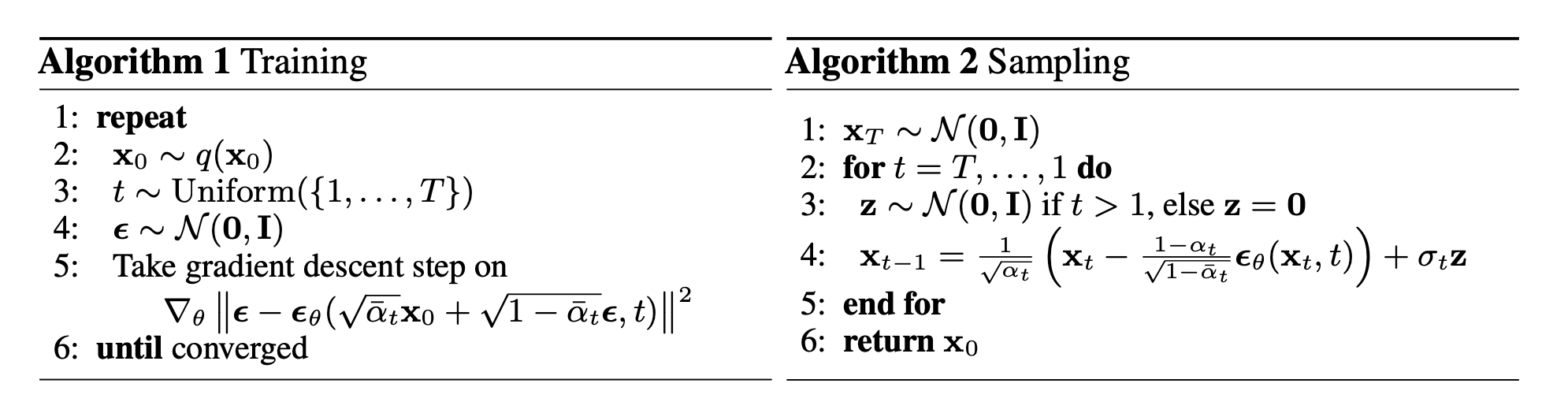
forward와 loss를 구하는 부분입니다. forward에서는 먼저 random int를 [1, timesteps]범위에서 batch size만큼 uniform distribution에서 뽑습니다. 그 후 image를 normalize하고 p_losses라는 함수에 img, t를 같이 넣어줍니다.

 

p_losses에서는 noise를 먼저 normal gaussian distribution에서 sampling합니다. 그리고   

\( \epsilon_{offset}=\epsilon+\sigma \cdot\mathcal{N}(0, I) \)를 통해 offset noise라는 기법을 noise에 적용해줍니다. offsret noise를 추가하여 학습 과정에서 노이즈를 더 안정적으로 예측할 수 있게 됩니다. 그 후, q_sample이라는 함수에 img(x_start)이전에 sampling한 t, noise를 인자로 주어 \(x_t\)를 만듭니다.

 

이전에 본 Unet(model)에 \(x_t, t\)를 주어 model_out을 뽑아냅니다. 참고로 model_out은 논문상으로는 \(\epsilon_{t}\)이지만 경우에따라서 \(x_0\)이나 velocity가 될 수 있다고 위에서 말했었습니다. 그 이유로, 분기문으로 objective에 따른 mse계산을 위해 target을 선택합니다. 그리고 model의 결과와 target으로 mse를 구하고 batch차원으로 싹다 평균낸 후, 위에서 loss_weight를 정의했는데 이를 적용시켜준 후 해당 loss값을 반환합니다.

 

p_losses에서 \(x_t\)계산에 사용된 q_sample에서는 \(\sqrt{\bar{\alpha}_t}x_0+\sqrt{1-\bar{\alpha}_t}\epsilon\)을 통해 \(x_t\)를 구합니다. 참고로 q_sample에 있는 immiscible은 만약 특정 데이터가 지나치게 강한 노이즈를 받거나, 특정 노이즈 패턴이 학습되지 않는 경우 적용할 수 있는 방법입니다.

    def model_predictions(self, x, t, x_self_cond = None, clip_x_start = False, rederive_pred_noise = False):
        model_output = self.model(x, t, x_self_cond)
        maybe_clip = partial(torch.clamp, min = -1., max = 1.) if clip_x_start else identity

        if self.objective == 'pred_noise':
            pred_noise = model_output
            x_start = self.predict_start_from_noise(x, t, pred_noise)
            x_start = maybe_clip(x_start)

            if clip_x_start and rederive_pred_noise:
                pred_noise = self.predict_noise_from_start(x, t, x_start)

        elif self.objective == 'pred_x0':
            x_start = model_output
            x_start = maybe_clip(x_start)
            pred_noise = self.predict_noise_from_start(x, t, x_start)

        elif self.objective == 'pred_v':
            v = model_output
            x_start = self.predict_start_from_v(x, t, v)
            x_start = maybe_clip(x_start)
            pred_noise = self.predict_noise_from_start(x, t, x_start)

        return ModelPrediction(pred_noise, x_start)
        

    def predict_start_from_noise(self, x_t, t, noise):
        return (
            extract(self.sqrt_recip_alphas_cumprod, t, x_t.shape) * x_t -
            extract(self.sqrt_recipm1_alphas_cumprod, t, x_t.shape) * noise
        )

p_losses에서 model에 입력을 주입할때 사용한 model_prediction입니다. Unet에 집어넣어 model_output을 만들고, clamp로 [-1, 1]범위로 output의 출력값의 범위를 조절합니다. 그 후, 앞서 말했던 objective에 따라 x_start, pred_noise를 계산합니다. 예를들어, objective == pred_noise에서 pred_noise는 model_output 그 자체일 것이며, x_start는 predict_start_from_noise함수를 통해 \(x_0 = \frac{1}{\sqrt{\bar{\alpha}_t}}(x_{t}-\sqrt{1-\bar{\alpha}_t}\cdot\epsilon_{\theta}\)를 구합니다. 나머지 objective도 동일하게 계산할 수 있고, ModelPrediction이라는 새로운 tuple과같은 구조체로 반환합니다.

 

DDPM Sampling

    @torch.inference_mode()
    def sample(self, batch_size = 16, return_all_timesteps = False):
        (h, w), channels = self.image_size, self.channels
        sample_fn = self.p_sample_loop if not self.is_ddim_sampling else self.ddim_sample
        return sample_fn((batch_size, channels, h, w), return_all_timesteps = return_all_timesteps)
        
        
    # sampling
    @torch.inference_mode()
    def p_sample_loop(self, shape, return_all_timesteps = False):
        batch, device = shape[0], self.device

        # x_T는 랜덤 가우시안 노이즈
        img = torch.randn(shape, device = device)
        imgs = [img]

        x_start = None
        # t를 역순으로 시작해서 x_0까지 점진적으로 샘플을 복원
        for t in tqdm(reversed(range(0, self.num_timesteps)), desc = 'sampling loop time step', total = self.num_timesteps):
            
            # self-cond가 켜져있으면, 이전의 x_start값을 다음 단계의 추가 입력으로 사용
            self_cond = x_start if self.self_condition else None
            img, x_start = self.p_sample(img, t, self_cond)
            imgs.append(img)

        ret = img if not return_all_timesteps else torch.stack(imgs, dim = 1)

        # 데이터를 [0, 1]범위로 변환 (DDM 학습시에 [-1, 1]범위로 학습했음)
        ret = self.unnormalize(ret)
        return ret
        
    # 현재 시간 t에서 x_t -> x_t-1을 샘플링
    @torch.inference_mode()
    def p_sample(self, x, t: int, x_self_cond = None):
        # 현재 배치 크기와 디바이스를 가져옴
        b, *_, device = *x.shape, self.device

        # 모든 배치에대해 현재 t값을 동일한 형태로 변환해줌
        batched_times = torch.full((b,), t, device = device, dtype = torch.long)

        # 모델이 예측한 x_t-1의 평균값과 분산을 활용
        model_mean, _, model_log_variance, x_start = self.p_mean_variance(
            x = x, t = batched_times, x_self_cond = x_self_cond, clip_denoised = True)
        noise = torch.randn_like(x) if t > 0 else 0. # no noise if t == 0

        # x_t-1샘플링을 mu + sigma * noise 형식으로 진행함
        pred_img = model_mean + (0.5 * model_log_variance).exp() * noise
        
        
    def p_mean_variance(self, x, t, x_self_cond = None, clip_denoised = True):
        preds = self.model_predictions(x, t, x_self_cond)
        x_start = preds.pred_x_start

        if clip_denoised:
            x_start.clamp_(-1., 1.)

        model_mean, posterior_variance, posterior_log_variance = self.q_posterior(x_start = x_start, x_t = x, t = t)
        return model_mean, posterior_variance, posterior_log_variance, x_start
        return pred_img, x_start
        
        
    def q_posterior(self, x_start, x_t, t):
        posterior_mean = (
            extract(self.posterior_mean_coef1, t, x_t.shape) * x_start +
            extract(self.posterior_mean_coef2, t, x_t.shape) * x_t
        )
        posterior_variance = extract(self.posterior_variance, t, x_t.shape)
        posterior_log_variance_clipped = extract(self.posterior_log_variance_clipped, t, x_t.shape)

        
        return posterior_mean, posterior_variance, posterior_log_variance_clipped

sample함수에서는 sample_fn을 is_ddim_sampling에 따라서 ddpm sampling을 할것인지, ddim sampling을 할것인지로 나눕니다. 그리고 ddpm의 경우에는 p_sample_loop으로 결과를 반환하게 됩니다.

 

p_sample_loop에서 우선 img를 랜덤 가우시안 노이즈로 설정합니다. 그 후, t를 역순으로 시작하여 img를 점진적으로 timestep만큼 반복하여 sampling을 합니다. 반복문 안에서 p_sample함수를 통해 추정한 \(x_{t-1}, x_{0}\)을 뽑아내고 img배열에 붙힙니다. 그 후, 복원한 sample을 unnormalize시켜 반환합니다.

 

p_sample은 \(x_t \rightarrow x_{t-1} \)를 하는 과정입니다. 일단 모든 batch만큼 현재 timestep(t)값으로 채운 배열을 만듭니다. t를 통해 모든 batch에 대해 p_mean_variance함수를 통해 model_mean, model_log_variance, x_start를 구합니다. 그리고 noise를 샘플링하고 \(x_{t-1} = \mu + (\frac{1}{2}log(\sigma^{2})\epsilon\)식을 통해 \(x_{t-1}\)의 pred_img를 sampling합니다.

 

p_sample에서 사용된 p_mean_variance는 \(x_t\), t를 통해 preds를 만들고, x_start(=\(x_0\))과 함께 q_posterior에 투입하여 model_mean, posterior_variance, posterior_log_variance를 구합니다. q_posterior에 사용된 변수들은 위에서 언급한 register buffer에 저장했던 posterior_log_variance_clipped, posterior_mean_coef1, posterior_mean_coef2입니다.

 

DDIM Sampling

    # ddim은 deterministic하게 sampling가능
    @torch.inference_mode()
    def ddim_sample(self, shape, return_all_timesteps = False):
        # eta: stochasticity조절 변수 (0이면 DDPM과 동일), objective: 모델이 예측하는 대상(pred_x0, pred_noise, pred_v...)
        batch, device, total_timesteps, sampling_timesteps, eta, objective = shape[0], self.device, self.num_timesteps, self.sampling_timesteps, self.ddim_sampling_eta, self.objective

        
        # ex) T=1000, sampling_timesteps=50 --> time_pairs [(999, 980), (880, 960), ..., (40, 20), (20, 0)]
        times = torch.linspace(-1, total_timesteps - 1, steps = sampling_timesteps + 1)   # [-1, 0, 1, 2, ..., T-1] when sampling_timesteps == total_timesteps
        times = list(reversed(times.int().tolist()))
        time_pairs = list(zip(times[:-1], times[1:])) # [(T-1, T-2), (T-2, T-3), ..., (1, 0), (0, -1)]

        # img는 gaussian noise로 시작
        img = torch.randn(shape, device = device)
        imgs = [img]

        # self-conditioning도 가능
        x_start = None

        for time, time_next in tqdm(time_pairs, desc = 'sampling loop time step'):
            time_cond = torch.full((batch,), time, device = device, dtype = torch.long)
            # self-conditioning이 활성화되면, 이전에 예측한 x_0을 현재 스텝에서 입력으로 활용
            self_cond = x_start if self.self_condition else None

            # model이 x_t로부터 x_0과 noise를 예측
            pred_noise, x_start, *_ = self.model_predictions(img, time_cond, self_cond, clip_x_start = True, rederive_pred_noise = True)

            # 마지막 timestep에서는 x_0을 직접 반환
            if time_next < 0:
                img = x_start
                imgs.append(img)
                continue
            
            # 𝛼_t
            alpha = self.alphas_cumprod[time]
            # 𝛼_t-1
            alpha_next = self.alphas_cumprod[time_next]

            # sigma를 아래와같이 설정하면 forward-process가 Markovian이 되어 generative(reverse-process)가 DDPM이 된다.
            # sigma = 0이면 x_t-1, x_0에 대하여 forward process가 deterministic DDIM이 된다.
            # 참고 (DDPM의 목적함수로 학습된 implicit probablistic model이기 때문에 DDIM이라 부른다.)
            sigma = eta * ((1 - alpha / alpha_next) * (1 - alpha_next) / (1 - alpha)).sqrt()

            # 스케일링 계수 (Noise term을 조절)
            c = (1 - alpha_next - sigma ** 2).sqrt()

            noise = torch.randn_like(img)

            img = x_start * alpha_next.sqrt() + \
                  c * pred_noise + \
                  sigma * noise

            imgs.append(img)

        ret = img if not return_all_timesteps else torch.stack(imgs, dim = 1)

        ret = self.unnormalize(ret)
        return ret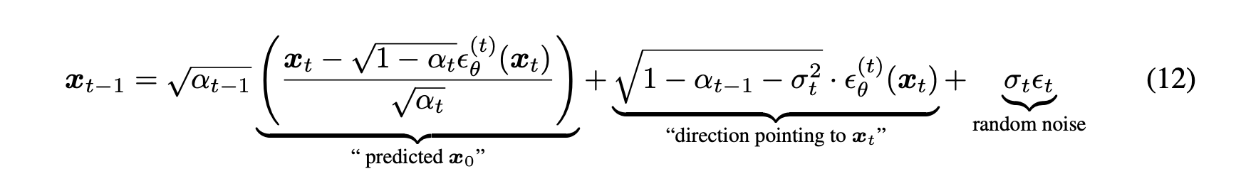

ddim sampling

DDIM은 ddpm과 objective의 최적해가 같다고 증명되었고, forward process를 non-Markovian process로 바꾸어 sampling acceleration이 가능한 ICCV2021에 소개된 논문입니다. 대게 ddpm으로 훈련된 모델을 ddim으로 샘플링해 샘플링만을 가속화하고 샘플링 퀄리티를 높일수 있습니다.

meaning of ddim sigma value

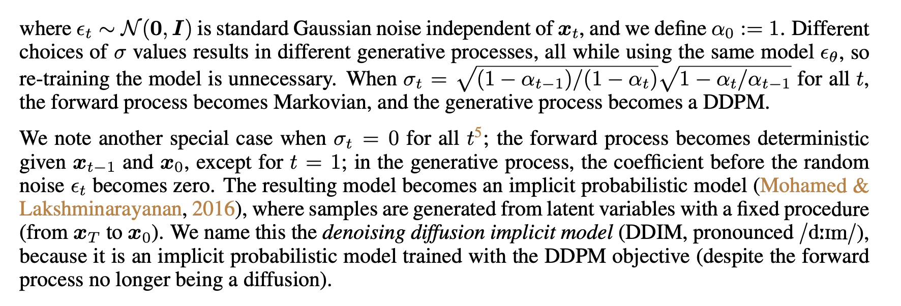
ddim에서 eta는 \(\sigma_t\)를 말하는 것이며 이를 조절하여 ddim을 ddpm으로 만들 수도 있습니다. ddim sampling도 ddpm처럼 img를 gaussian noise로 놓고 시작합니다. 그리고 time_pairs를 따로 정의하는데 이는 sampling acceleration을 위해 미리 sampling timestep으로 timestep을 쪼갠 배열입니다. 그 후, model_prediction으로 ddpm과 동일하게 pred_noise, x_start를 만듭니다. 다음으로 alpha, alpha_next를 현재 timestep을 기반으로 만듭니다.

 

위에 ddim paper를 보면 모든 t에 대해 \(\sigma_t = \sqrt{(1-\alpha_{t-1})/(1-\alpha_t)}\sqrt{1-\alpha_{t}/\alpha_{t-1}}\)로 설정하면 forward process는 Markovian이 되어 generative process가 DDPM이 된다고 되어있습니다(ddpm에서의 \(\bar{\alpha}=\alpha\)). 이를 기반으로 코드에서도 sigma를 위의 값과 eta의 곱으로 설정합니다. 그리고 noise term을 조절하는 스케일링 계수도 \(c = \sqrt{1-\alpha_{t-1}-\sigma^{2}}\)로 설정합니다(eq12에서의 "direction pointing to \(x_t\)"). 이제 img를 위 식들을 조합해서 만들어 내고, 결괏값(ret)의 배열을 unnormalize해서 반환합니다.

 

Trainer

# trainer class

class Trainer:
    def __init__(
        self,
        diffusion_model,
        folder,
        *,
        train_batch_size = 16,
        gradient_accumulate_every = 1,
        augment_horizontal_flip = True, # 이미지가 확률적으로 좌우반전 됨.
        train_lr = 1e-4,
        train_num_steps = 100000,
        ema_update_every = 10,
        ema_decay = 0.995,
        adam_betas = (0.9, 0.99),
        save_and_sample_every = 1000,
        num_samples = 25,
        results_folder = './results',
        amp = False,
        mixed_precision_type = 'fp16',
        split_batches = True,
        convert_image_to = None,
        calculate_fid = True,
        inception_block_idx = 2048,
        max_grad_norm = 1.,
        num_fid_samples = 50000,
        save_best_and_latest_only = False
    ):
        super().__init__()

        # accelerator

        self.accelerator = Accelerator(
            split_batches = split_batches,
            mixed_precision = mixed_precision_type if amp else 'no'
        )

        # model

        self.model = diffusion_model
        self.channels = diffusion_model.channels
        is_ddim_sampling = diffusion_model.is_ddim_sampling

        # default convert_image_to depending on channels

        if not exists(convert_image_to):
            convert_image_to = {1: 'L', 3: 'RGB', 4: 'RGBA'}.get(self.channels)

        # sampling and training hyperparameters

        assert has_int_squareroot(num_samples), 'number of samples must have an integer square root'
        self.num_samples = num_samples
        self.save_and_sample_every = save_and_sample_every

        self.batch_size = train_batch_size
        self.gradient_accumulate_every = gradient_accumulate_every
        assert (train_batch_size * gradient_accumulate_every) >= 16, f'your effective batch size (train_batch_size x gradient_accumulate_every) should be at least 16 or above'

        self.train_num_steps = train_num_steps
        self.image_size = diffusion_model.image_size

        self.max_grad_norm = max_grad_norm

        # dataset and dataloader

        self.ds = Dataset(folder, self.image_size, augment_horizontal_flip = augment_horizontal_flip, convert_image_to = convert_image_to)

        assert len(self.ds) >= 100, 'you should have at least 100 images in your folder. at least 10k images recommended'

        dl = DataLoader(self.ds, batch_size = train_batch_size, shuffle = True, pin_memory = True, num_workers = cpu_count())

        dl = self.accelerator.prepare(dl)
        self.dl = cycle(dl)

        # optimizer

        self.opt = Adam(diffusion_model.parameters(), lr = train_lr, betas = adam_betas)

        # for logging results in a folder periodically

        if self.accelerator.is_main_process:
            # diffusion_model의 가중치를 부드럽게 업데이트 해주기 위함
            self.ema = EMA(diffusion_model, beta = ema_decay, update_every = ema_update_every)
            self.ema.to(self.device)

        self.results_folder = Path(results_folder)
        self.results_folder.mkdir(exist_ok = True)

        # step counter state

        self.step = 0

        # prepare model, dataloader, optimizer with accelerator

        self.model, self.opt = self.accelerator.prepare(self.model, self.opt)

        # FID-score computation

        self.calculate_fid = calculate_fid and self.accelerator.is_main_process

        if self.calculate_fid:
            from denoising_diffusion_pytorch.fid_evaluation import FIDEvaluation

            if not is_ddim_sampling:
                self.accelerator.print(
                    "WARNING: Robust FID computation requires a lot of generated samples and can therefore be very time consuming."\
                    "Consider using DDIM sampling to save time."
                )

            self.fid_scorer = FIDEvaluation(
                batch_size=self.batch_size,
                dl=self.dl,
                sampler=self.ema.ema_model,
                channels=self.channels,
                accelerator=self.accelerator,
                stats_dir=results_folder,
                device=self.device,
                num_fid_samples=num_fid_samples,
                inception_block_idx=inception_block_idx
            )

        if save_best_and_latest_only:
            assert calculate_fid, "`calculate_fid` must be True to provide a means for model evaluation for `save_best_and_latest_only`."
            self.best_fid = 1e10 # infinite

        self.save_best_and_latest_only = save_best_and_latest_only
        
        

# dataset classes

class Dataset(Dataset):
    def __init__(
        self,
        folder,
        image_size,
        exts = ['jpg', 'jpeg', 'png', 'tiff'],
        augment_horizontal_flip = False,
        convert_image_to = None
    ):
        super().__init__()
        self.folder = folder
        self.image_size = image_size
        self.paths = [p for ext in exts for p in Path(f'{folder}').glob(f'**/*.{ext}')]

        maybe_convert_fn = partial(convert_image_to_fn, convert_image_to) if exists(convert_image_to) else nn.Identity()

        self.transform = T.Compose([
            T.Lambda(maybe_convert_fn),
            T.Resize(image_size),
            T.RandomHorizontalFlip() if augment_horizontal_flip else nn.Identity(),
            T.CenterCrop(image_size),
            T.ToTensor() # 범위를 0~1로 바꿔주는 역할도함 --> [-1, 1] (norm, train) --> [0, 1] (unorm, sample)
        ])

    def __len__(self):
        return len(self.paths)

    def __getitem__(self, index):
        path = self.paths[index]
        img = Image.open(path)
        return self.transform(img)

Trainer의 변수 설정 부분입니다. Dataset에 대하여 dataloader를 작성해줍니다. Dataset class를 잠깐보면, transform함수들이 작성되어있는데, Resize -> RandomHorizontalFlip -> CenterCrop -> ToTensor순으로 진행됩니다. dataloader또한, 분산 gpu처리를 가능하게 하기위해 accelerator에 등록해줍니다. Optimizer는 Adam을 씁니다. 그 다음으로accelerator.is_main_process(분산 환경에서 단 한번만 실행하기) 안에 EMA가 정의되어있는데, 이는 diffusion_model의 가중치를 부드럽게 업데이트해주기 위함입니다(현재 가중치를 더 많이 반영).

 

calculate_fid가 true라면 FIDEvaluation을 정의하여, 실제 dataset에서 num_fid_sample개의 sample을 뽑아 ground truth와 FID를 계산합니다. 첨언으로 직접 훈련시킬때 Trainer에 num_fid_sample을 32 * 10으로 줄건데, 이는 [32, 32, ..., 32]의 배열을 만들어 batch개의 sample을 만들고 inception_feature를 이를 통해 추출한 뒤 32 * 10개의 feature를 활용해 FID를 구해 반환하겠다는 의미입니다.

    def train(self):
        accelerator = self.accelerator
        device = accelerator.device

        with tqdm(initial = self.step, total = self.train_num_steps, disable = not accelerator.is_main_process) as pbar:

            while self.step < self.train_num_steps:
                self.model.train()

                total_loss = 0.

                # gradient_accumulate는 batch_Size가 큰 것을 simulation하기 위해 사용됨.
                for _ in range(self.gradient_accumulate_every):
                    # dataloader에서 한 배치의 데이터를 가져와서 GPU로 이동
                    data = next(self.dl).to(device)

                    # AMP를 사용하여 FP16연산을 자동으로 수행해주도록 해주는 함수
                    with self.accelerator.autocast():
                        loss = self.model(data)
                        # gradient_accumulate_every만큼의 가중치를 한번만 update해야하므로
                        loss = loss / self.gradient_accumulate_every
                        total_loss += loss.item()
                    
                    # FP16, multi-GPU, gradient-accumulation을 자동처리하면서 역전파
                    self.accelerator.backward(loss)

                # loss를 step1개 마다 보여줌
                pbar.set_description(f'loss: {total_loss:.4f}')

                accelerator.wait_for_everyone()
                # gradient cliping을 통해 gradient를 normalization해서 학습 안정성을 높임
                accelerator.clip_grad_norm_(self.model.parameters(), self.max_grad_norm)

                self.opt.step()
                # optimizer의 그래디언트 값을 초기화 하는 역할
                self.opt.zero_grad()

                accelerator.wait_for_everyone()

                self.step += 1


                if accelerator.is_main_process:
                    self.ema.update()

                    # 일정한 step마다 sampling 및 모델 저장을 실행하는 역할
                    if self.step != 0 and divisible_by(self.step, self.save_and_sample_every):
                        # ema를 비활성화
                        self.ema.ema_model.eval()

                        # autograd끔 (메모리 최적화)
                        with torch.inference_mode():
                            milestone = self.step // self.save_and_sample_every
                            # 샘플을 여러 배치로 나누는 과정
                            batches = num_to_groups(self.num_samples, self.batch_size)
                            
                            # sample을 수행 --> p_sample_loop()
                            all_images_list = list(map(lambda n: self.ema.ema_model.sample(batch_size=n), batches))

                        all_images = torch.cat(all_images_list, dim = 0)

                        # 25개 이미지만 sampling하는 것임
                        utils.save_image(all_images, str(self.results_folder / f'sample-{milestone}.png'), nrow = int(math.sqrt(self.num_samples)))

                        # whether to calculate fid

                        # FID 계산 -> 실제 이미지와 생성된 이미지가 얼마나 유사한지 평가
                        if self.calculate_fid:
                            fid_score = self.fid_scorer.fid_score() # *********병목**********
                            accelerator.print(f'fid_score: {fid_score}')

                        # FID 기준으로 이전보다 좋으면 best model로서 저장
                        if self.save_best_and_latest_only:
                            if self.best_fid > fid_score:
                                self.best_fid = fid_score
                                self.save("best")
                            self.save("latest")
                        else:
                            self.save(milestone)

                pbar.update(1)

        accelerator.print('training complete')

대부분의 코드를 주석으로 달았으므로 중요한 부분 몇개만 보겠습니다. 초반에 gradient_accumulate_every변수만큼 반복문을 돌아 data를 가져오고 loss를 gradient_accumulate_every만큼 나누어 backward를 하여 가중치를 누정한 후, opt.step()으로 반복문을 마치고 그 다음에 가중치를 업데이트 합니다. 이로 인해 마치 큰 배치를 학습하는 효과를 낼 수 있습니다.

 

마지막 부분에 step이 save_and_sample_every에 divisible가능하다면 num_samples개의 sample을 만들어 all_images에 concatenate합니다. 그리고 이를 milestone형태로 저장합니다. 그 후, calculate_fid가 True라면 위에서 정의한 fid_scorer.fid_score()를 통해 num_fid_samples만큼의 sample을 통해 FID를 계산하고, 이 점수를 기반으로 하여 만약 save_best_and_latest_only가 True라면 best fid를 가지는 모델을 저장합니다. 

 

Experiment

import kagglehub
import os
from torchvision import transforms
from torch.utils.data import Dataset, DataLoader
from PIL import Image
import torch
from denoising_diffusion_pytorch import Unet, GaussianDiffusion, Trainer
from torchvision import transforms as T, utils
import math

# Download latest version
path = kagglehub.dataset_download("jessicali9530/celeba-dataset")

print("Path to dataset files:", path)

model = Unet(
    dim = 64,
    dim_mults = (1, 2, 2), # [64, 64, 128, 128]
    flash_attn = False
)

diffusion = GaussianDiffusion(
    model,
    image_size = 64,
    timesteps = 1000,    # T --> time step
    sampling_timesteps=500, # ddim sampling을 활용
    beta_schedule = 'linear',
)

trainer = Trainer(
    diffusion,
    os.path.join(path, "img_align_celeba/img_align_celeba"),
    train_batch_size = 32,
    train_lr = 1e-4,
    train_num_steps = 100000,         # total training steps
    gradient_accumulate_every = 2,    # gradient accumulation steps
    ema_decay = 0.995,                # exponential moving average decay
    amp = True,                       # turn on mixed precision
    calculate_fid = True,              # whether to calculate fid during training
    num_fid_samples = 32 * 10,
    save_best_and_latest_only=True # 가장 best fid를 가지는 model을 milestone으로 저장하겠다.
)

# trainer.train()

trainer.load(100)

num_samples = 64
all_images_list = list(map(lambda n: trainer.ema.ema_model.sample(batch_size=n), [32, 32]))
all_images = torch.cat(all_images_list, dim = 0)

utils.save_image(all_images, "./results/sample-100-test.png", nrow = int(math.sqrt(num_samples)))

• dataset: celeba
• GaussianDiffusion
  • image_size: 64
  • timesteps: 1000
  • sampling_timestep: 500 (ddim)
    • ddpm의 2배 속도로 accelerate했다는 의미
  • beta_schedule: linear (default = sigmoid)
• Trainer
  
  • train_batch_size: 32
  • train_lr: 0.004
  • train_num_steps: 100K
  • gradient_accumulate_every: 2 (사실상 batch_size = 64를 simulation)
  • ema_decay: 0.995
  • num_fid_samples: 320

sampling result

 

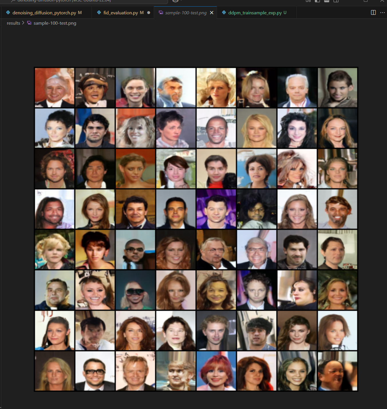
4090 1way로 대략 10시간정도 train을 한 후, 가장 best model의 checkpoint에서 무작위 noise 64개로부터 sampling한 결과입니다. 

 

이 외에도 latent vector(noise)가 같을때 결과가 어떤지와 semantic interpolation등도 실험해보고 싶었지만, 시간관계상 다음에 여유가 될때 한번 해보겠습니다.