![[ 딥러닝 최신 알고리즘 - PRMI Lab ] - ViT 구현과, huggingface를 이용한 fine-tuning](https://img1.daumcdn.net/thumb/R750x0/?scode=mtistory2&fname=https%3A%2F%2Fblog.kakaocdn.net%2Fdn%2FbeKiYb%2FbtsC2AxhMWm%2FUy9eQLIm9CbGKF1wlnHBPk%2Fimg.png)
https://github.com/eunoiahyunseo/rofydeo-model-archiving/tree/main/models/ViT
해당 github 주소에 코드들은 올려 놓았습니다.
모델 구현
# pytocrh와 기타 util라이브러리를 import해온다. import torch import torch.nn.functional as F import matplotlib.pyplot as plt from torch import nn from torch import Tensor from PIL import Image from torchvision.transforms import Compose, Resize, ToTensor # 텐서의 차원관리를 해주는, einops from einops import rearrange, reduce, repeat from einops.layers.torch import Rearrange, Reduce # pytorch모델의 구조도와 요약을 확인할 수 있다. from torchsummary import summary
위와같이 구현에 필요한 모듈들을 불러와줍니다. 여기서 우리는 텐서의 차원관리를 einops를 통해 해보겠습니다. 한번 사용해보니까 매우 편하고 앞으로 애용하게 될 것 같습니다.
Patch Embedding
class PatchEmbedding(nn.Module): def __init__(self, in_channels: int = 3, patch_size: int = 16, emb_size: int = 768): self.patch_size = patch_size super().__init__() self.projection = nn.Sequential( # ViT논문에서는 Conv2d를 사용하는게, Linear레이어 하나를 더 추가하는 것보다 더 계산 효율적이라고 했음 # 최종적으로 [batch_size, (h//patch_size)*(w//patch_size), embed_size)]크기의 텐서가 된다. nn.Conv2d(in_channels, emb_size, kernel_size=patch_size, stride=patch_size), Rearrange('b e (h) (w) -> b (h w) e') # Rearrange('b c (h s1) (w s2) -> b (h w) (s1 s2 c)', s1=patch_size, s2=patch_size), # nn.Linear(patch_size * patch_size * in_channels, emb_size) # linear projection ) def forward(self, x: Tensor) -> Tensor: x = self.projection(x) return x PatchEmbedding()(x).shape
patchEmbedding을 우선 구현한 부분입니다. 이는 학습 가능한 행렬로서 emb_size로 patch의 sequence들을 투영시킵니다. 하지만 논문의 Appendix에 구현상으로는 Conv2d를 쓰는 것이 더욱 계산 효율적이라고 되어있습니다.
CLS TOKEN
class PatchEmbedding(nn.Module): def __init__(self, in_channels: int = 3, patch_size: int = 16, emb_size: int = 768): self.patch_size = patch_size super().__init__() self.projection = nn.Sequential( # ViT논문에서는 Conv2d를 사용하는게, Linear레이어 하나를 더 추가하는 것보다 더 계산 효율적이라고 했음 # 최종적으로 [batch_size, (h//patch_size)*(w//patch_size), embed_size)]크기의 텐서가 된다. nn.Conv2d(in_channels, emb_size, kernel_size=patch_size, stride=patch_size), Rearrange('b e (h) (w) -> b (h w) e') # Rearrange('b c (h s1) (w s2) -> b (h w) (s1 s2 c)', s1=patch_size, s2=patch_size), # nn.Linear(patch_size * patch_size * in_channels, emb_size) # linear projection ) # nn.parameter는 모델에 학습 가능한 파라미터를 추가할 때 텐서로 추가하는 방법이다. self.cls_token = nn.Parameter(torch.randn(1, 1, emb_size)) def forward(self, x: Tensor) -> Tensor: b, _, _, _ = x.shape x = self.projection(x) cls_token = repeat(self.cls_token, '() n e -> b n e', b=b) x = torch.cat([cls_token, x], dim=1) return x PatchEmbedding()(x).shape
CLS TOKEN을 추가해주었습니다. nn.Parameter로 학습가능한 가중치로서 모델에 z0부분에 추가해줍니다. 제가 주석으로 코드의 결과의 행렬 사이즈를 상세히 서술했으니 참고하시길 바랍니다.
POSITION EMBEDDING
class PatchEmbedding(nn.Module): def __init__(self, in_channels: int = 3, patch_size: int = 16, emb_size: int = 768, img_size: int = 224): self.patch_size = patch_size super().__init__() self.projection = nn.Sequential( # ViT논문에서는 Conv2d를 사용하는게, Linear레이어 하나를 더 추가하는 것보다 더 계산 효율적이라고 했음 # 최종적으로 [batch_size, (h//patch_size)*(w//patch_size), embed_size)]크기의 텐서가 된다. nn.Conv2d(in_channels, emb_size, kernel_size=patch_size, stride=patch_size), Rearrange('b e (h) (w) -> b (h w) e') # Rearrange('b c (h s1) (w s2) -> b (h w) (s1 s2 c)', s1=patch_size, s2=patch_size), # nn.Linear(patch_size * patch_size * in_channels, emb_size) # linear projection ) # nn.parameter는 모델에 학습 가능한 파라미터를 추가할 때 텐서로 추가하는 방법이다. self.cls_token = nn.Parameter(torch.randn(1, 1, emb_size)) self.positions = nn.Parameter(torch.randn((img_size // patch_size) ** 2 + 1, emb_size)) def forward(self, x: Tensor) -> Tensor: b, _, _, _ = x.shape x = self.projection(x) cls_token = repeat(self.cls_token, '() n e -> b n e', b=b) x = torch.cat([cls_token, x], dim=1) x += self.positions return x PatchEmbedding()(x).shape
learnable한 position embedding을 추가해줍니다. 논문에 나와있는 수치 그대로를 nn.Parameter로 정의해주고 그대로 이전 결괏값과 더해줍니다. 이는 패치의 위치정보를 ViT에서 확실히 학습할 수 있게됩니다.
Transformer
''' 원래 트랜스포머에서 Wq, Wk, Wv 벡터의 차원은 d_model보다 작은 차원을 갖는다. [emb_size, d_model // num_heads]의 차원을 가지고 추후에 MSA의 끝단에서 concatenate하게 된다. ''' class MultiHeadAttention(nn.Module): def __init__(self, emb_size: int = 768, num_heads: int = 8, dropout: float = 0): super().__init__() self.emb_size = emb_size self.num_heads = num_heads self.keys = nn.Linear(emb_size, emb_size) self.queries = nn.Linear(emb_size, emb_size) self.values = nn.Linear(emb_size, emb_size) self.att_drop = nn.Dropout(dropout) self.projection = nn.Linear(emb_size, emb_size) self.scaling = (self.emb_size // num_heads) ** -0.5 def forward(self, x: Tensor, mask: Tensor = None) -> Tensor: # 위에서 말했던 것처럼 num_heads로 keys, queries, values를 쪼갠다. # [batch, heads, seq_len, emb_size] 크기의 텐서가 된다. # [1, 8, 197, 96] -> x는 나누기 전인 [1, 197, 768] queries = rearrange(self.queries(x), "b n (h d) -> b h n d", h=self.num_heads) keys = rearrange(self.keys(x), "b n (h d) -> b h n d", h=self.num_heads) values = rearrange(self.values(x), "b n (h d) -> b h n d", h=self.num_heads) # print('qureis shape -> ', queries.shape) # print('keys shape -> ', keys.shape) # print('values shape -> ', values.shape) # queries, keys를 이제 행렬곱 해주어야 한다. # 아래 코드와같이 하면 자동으로 transpose되고 내적이 된다. # [batch, heads, query_len, key_len] 크기의 텐서가 된다. # [1, 8, 197, 197] energy = torch.einsum('bhqd, bhkd -> bhqk', queries, keys) # print('energy shape -> ', energy.shape) if mask is not None: fill_value = torch.finfo(torch.float32).min # -max energy.mask_fill(~mask, fill_value) att = F.softmax(energy, dim=-1) * self.scaling # scaling된 attention score att = self.att_drop(att) # print('att shape -> ', att.shape) out = torch.einsum('bhal, bhlv -> bhav', att, values) out = rearrange(out, "b h n d -> b n (h d)") out = self.projection(out) return out patches_embedded = PatchEmbedding()(x) MultiHeadAttention()(patches_embedded).shape
transformer부분을 간단히 MSA부분만 구현해주었습니다.
Residual Network
class ResidualAdd(nn.Module): def __init__(self, fn): super().__init__() self.fn = fn def forward(self, x, **kwargs): res = x x = self.fn(x, **kwargs) x += res return x
ResNet구조를 구현했습니다.
MLP
class FeedForwardBlock(nn.Sequential): def __init__(self, emb_size: int, expansion: int = 4, drop_p: float = 0.): super().__init__( # upsample을 expansion ratio만큼 해주었음 원래 트랜스 포머에서도 d_model=512 -> dfff=2048 (expansion ratio = 4) nn.Linear(emb_size, expansion * emb_size), nn.GELU(), # Dropout은 원래 과적합이 일어나기 쉬운 Dense, Fully Connected Layer뒤에 적용하는 것이 일반적이다. # Attention Layer뒤에도 Dropout을 사용하는데, 이는 모델이 특정 헤드에 지나치게 의존하는 것을 방지한다. -> 위에 적용했음 nn.Dropout(drop_p), nn.Linear(expansion * emb_size, emb_size) )
MLP부분을 GELU activation function과 expansion ratio를 통해 bottle-neck구조로 만들어 주었습니다.
TransformerEncoderBlock
class TransformerEncoderBlock(nn.Sequential): def __init__(self, emb_size: int = 768, drop_p: float = 0, forward_expansion: int = 4, forward_drop_p: float = 0., **kwargs): super().__init__( ResidualAdd( nn.Sequential( nn.LayerNorm(emb_size), MultiHeadAttention(emb_size, **kwargs), nn.Dropout(drop_p))), ResidualAdd( nn.Sequential( nn.LayerNorm(emb_size), # layer normalization FeedForwardBlock( emb_size, expansion=forward_expansion, drop_p=forward_drop_p), nn.Dropout(drop_p))) ) patches_embedded = PatchEmbedding()(x) TransformerEncoderBlock()(patches_embedded).shape
Encoder Block을 nn.Sequential로 간단히 구현해줍니다.
TransformerEncoder
class TransformerEncoder(nn.Sequential): def __init__(self, depth: int = 12, **kwargs): super().__init__(*[TransformerEncoderBlock(**kwargs) for _ in range(depth)])
Encoder를 depth와함께 반복해 최종적으로 만들어줍니다.
Classification Head
class ClassificationHead(nn.Sequential): def __init__(self, emb_size: int = 768, n_classes: int = 1000): super().__init__( Reduce('b n e -> b e', reduction='mean'), nn.LayerNorm(emb_size), nn.Linear(emb_size, n_classes) )
classification head를 만들어줍니다.
ViT
class ViT(nn.Sequential): def __init__(self, in_channels: int = 3, patch_size: int = 16, emb_size: int = 768, img_size: int = 224, depth: int = 12, n_classes: int = 1000, **kwargs): super().__init__( PatchEmbedding(in_channels, patch_size, emb_size, img_size), TransformerEncoder(depth, emb_size=emb_size, **kwargs), ClassificationHead(emb_size, n_classes) )
만들어준 head까지 붙혀서 ViT를 만들어줍니다.
학습
https://arxiv.org/pdf/2112.13492.pdf
해당 논문을 기반으로 트랜스포머의 configuration을 설정했습니다.
import os import time from tqdm import tqdm import argparse import torchvision.transforms as tfs from torch.utils.data import DataLoader from timm.models.layers import trunc_normal_ from torchvision.datasets.cifar import CIFAR10 from torch.utils.tensorboard import SummaryWriter
늘 그렇듯, 필요한 코드를 불러오고, CIFAR10데이터셋에 대해 training을 50epoch만 시켜볼 것이므로 이와 관련된 모듈을 불러옵니다.
class ArgumentParser(): def __init__(self, epoch: int = 50, batch_size: int = 128, lr: float = 1e-3, step_size: int = 100, root: str = './CIFAR10', log_dir: str = './log', name: str = 'vit_cifar10', rank: int = 0): self.epoch = epoch self.batch_size = batch_size self.lr = lr self.step_size = step_size self.root = root self.log_dir = log_dir self.name = name self.rank = rank return
관련 파라미터들을 하나의 클래스에 때려박아주었습니다.
vit_cifar_input: dict = { "img_size": 32, "patch_size": 4, "n_classes": 10, "emb_size": 192, "forward_expansion": 2 } ops = ArgumentParser() # device 셋팅 device = torch.device('cuda:{}'.format(0) if torch.cuda.is_available() else 'cpu') # dataset / dataloader 정의를 해준다. transform_cifar = tfs.Compose([ tfs.RandomCrop(32, padding=4), tfs.RandomHorizontalFlip(), tfs.ToTensor(), tfs.Normalize(mean=(0.4914, 0.4822, 0.4465), std=(0.2023, 0.1994, 0.2010)) ]) train_set = CIFAR10(root=ops.root, train=True, download=True, transform=transform_cifar) test_set = CIFAR10(root=ops.root, train=False, download=True, transform=transform_cifar) train_loader = DataLoader(dataset=train_set, shuffle=True, batch_size=ops.batch_size) test_loader = DataLoader(dataset=test_set, shuffle=True, batch_size=ops.batch_size) # model 정의 model = ViT(**vit_cifar_input).to(device) # criterion 정의 criterion = nn.CrossEntropyLoss() # optimizer 정의 optimizer = torch.optim.Adam(model.parameters(), lr=ops.lr, weight_decay=5e-5) # scheduler 정의 scheduler = torch.optim.lr_scheduler.CosineAnnealingLR(optimizer, T_max=ops.epoch, eta_min=1e-5) # logger 정의 os.makedirs(ops.log_dir, exist_ok=True)
그리고 dataloader와, model, criterion, optimizer, scheduler, logger를 정의해줍니다.
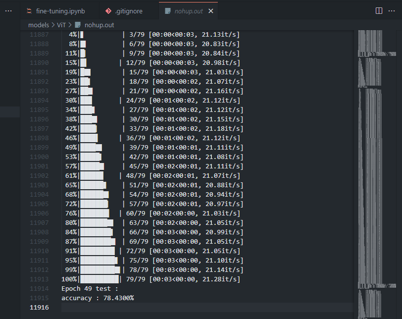
# training writer = SummaryWriter() print("training....") best_accuracy = 0.0 for epoch in range(ops.epoch): model.train() tic = time.time() for idx, (img, target) in enumerate(tqdm(train_loader)): img = img.to(device) # [N, 3, 32, 32] <- cifar with batch size target = target.to(device) # [N] output = model(img) # classification_head의 출력이니까 [N, 10] -> cifar10이니까 class=10 loss = criterion(output, target) # crossentropy 값 계산 -> 단순히 분류 문제이기 때문 optimizer.zero_grad() loss.backward() optimizer.step() for param_group in optimizer.param_groups: lr = param_group['lr'] if idx % ops.step_size == 0: writer.add_scalar('Training loss', loss, epoch * len(train_loader) + idx) print('Epoch : {}\t' 'step : [{}/{}]\t' 'loss : {}\t' 'lr : {}\t' 'time {}\t' .format(epoch, idx, len(train_loader), loss, lr, time.time() - tic)) save_path = os.path.join(ops.log_dir, ops.name, 'saves') os.makedirs(save_path, exist_ok=True) # test print('Validation of epoch[{}]'.format(epoch)) model.eval() correct = 0 val_avg_loss = 0 total = 0 with torch.no_grad(): for idx, (img, target) in enumerate(tqdm(test_loader)): img = img.to(device) target = target.to(device) output = model(img) loss = criterion(output, target) output = torch.softmax(output, dim=1) pred, idx_ = output.max(-1) correct += torch.eq(target, idx_).sum().item() total += target.size(0) val_avg_loss += loss.item() print('Epoch {} test : '.format(epoch)) accuracy = correct / total print("accuracy : {:.4f}%".format(accuracy * 100.)) val_avg_loss = val_avg_loss / len(test_loader) if epoch % 5 == 0 and accuracy > best_accuracy: best_accuracy = accuracy save_path = os.path.join(ops.log_dir, ops.name, 'saves') os.makedirs(save_path, exist_ok=True) checkpoint = { 'epoch': epoch, 'model_state_dict': model.state_dict(), 'optimizer_state_dict': optimizer.state_dict(), 'scheduler_state_dict': scheduler.state_dict(), 'best_accuracy': best_accuracy } torch.save(checkpoint, os.path.join(save_path, ops.name + '.{}.pth.tar'.format(epoch))) writer.add_scalar('Test loss', loss, epoch) writer.add_scalar('Tert accuracy', val_avg_loss, epoch) scheduler.step()
마지막으로 train 코드를 돌려줍니다. 그리고 ipynb파일을 python파일로 변경하고 background에서 모델을 돌려주어 tensorboard와 함께 모니터링 해주었습니다.
$jupyter nbconvert --to script {파일명}.ipynb $nohup python {파일명}.py &
이제 직접 학습시킨 모델을 통해 제가 다운받은 이미지를 예측시켜보도록 하겠습니다.
import matplotlib.pyplot as plt def display_image_with_label(img, label): plt.imshow(img ) plt.axis('off') # 축 제거 # 레이블(클래스 이름) 표시 plt.title(f"Predicted label: {label}") # 이미지와 레이블 함께 출력 plt.show() model = ViT(**vit_cifar_input) checkpoint_path = './log/vit_cifar10/saves/vit_cifar10.48.pth.tar' checkpoint = torch.load(checkpoint_path) model.load_state_dict(checkpoint['model_state_dict']) cifar10_transform = Compose([Resize((32, 32)), ToTensor()]) origin_img = Image.open('./image.jpg') # 분류하고자 하는 이미지 파일 img = cifar10_transform(origin_img) img = img.unsqueeze(0) # 배치 차원 추가 with torch.no_grad(): # 그래디언트 계산 비활성화 model.eval() outputs = model(img) _, predicted = torch.max(outputs, 1) classes = [ "airplane", # 비행기 "automobile", # 자동차 "bird", # 새 "cat", # 고양이 "deer", # 사슴 "dog", # 개 "frog", # 개구리 "horse", # 말 "ship", # 배 "truck" # 트럭 ] display_image_with_label(origin_img, classes[predicted[0]])
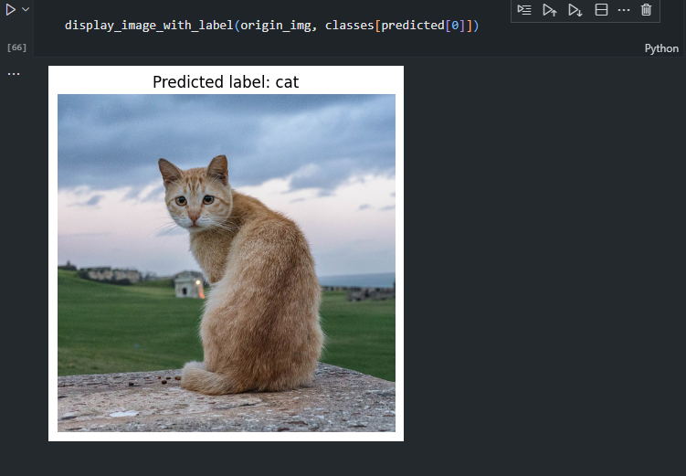
ViT로 정확도는 좀 낮지만, 잘 분류하는 것을 볼 수 있습니다.
그 외에도 hugging space를 이용해 fine-tuning한 코드도 있으니 한번 git들어가서 확인해보시길 바랍니다!
'AIML > 딥러닝 최신 트렌드 알고리즘' 카테고리의 다른 글
| [ 딥러닝 최신알고리즘 - PRMI Lab ] - DeiT (data-efficient image transformers & distillation through attention) (1) | 2024.01.12 |
|---|---|
| [ 딥러닝 최신 알고리즘 - PRMI Lab ] - KD: Knowledge Distillation (0) | 2024.01.08 |
| [ 딥러닝 최신 알고리즘 - PRMI Lab ] - ViT: Vision Transformer(2021) (1) | 2024.01.06 |
| [ 딥러닝 최신 트랜드 - PRMI Lab ] - Variations of Transformers (0) | 2023.08.06 |
| [ 딥러닝 구현 - PRMI Lab ] - 트랜스포머(Transformer)의 구현 (0) | 2023.08.03 |